Data Science
Basic Models
- Required files:
test_plan.py
#!/usr/bin/env python
"""
This example shows how to display various data modelling techniques and their
associated statistics in Testplan. The models used are:
* linear regression
* classification
* clustering
"""
import os
import sys
import random
from testplan import test_plan
from testplan.testing.multitest import MultiTest
from testplan.testing.multitest.suite import testsuite, testcase
from testplan.report.testing.styles import Style
from sklearn.model_selection import train_test_split
from sklearn.metrics import mean_squared_error, r2_score, classification_report
from sklearn.cluster import KMeans
from sklearn import datasets, linear_model, svm
import matplotlib
matplotlib.use("agg")
import matplotlib.pyplot as plot
import numpy as np
def create_scatter_plot(title, x, y, x_label, y_label, c=None):
plot.scatter(x, y, c=c)
plot.grid()
plot.xlabel(x_label)
plot.ylabel(y_label)
plot.title(title)
def create_image_plot(title, img_data, rows, columns, index):
plot.subplot(rows, columns, index)
plot.axis("off")
plot.imshow(img_data, cmap=plot.cm.gray_r, interpolation="nearest")
plot.title(title)
@testsuite
class ModelExamplesSuite:
@testcase
def basic_linear_regression(self, env, result):
"""
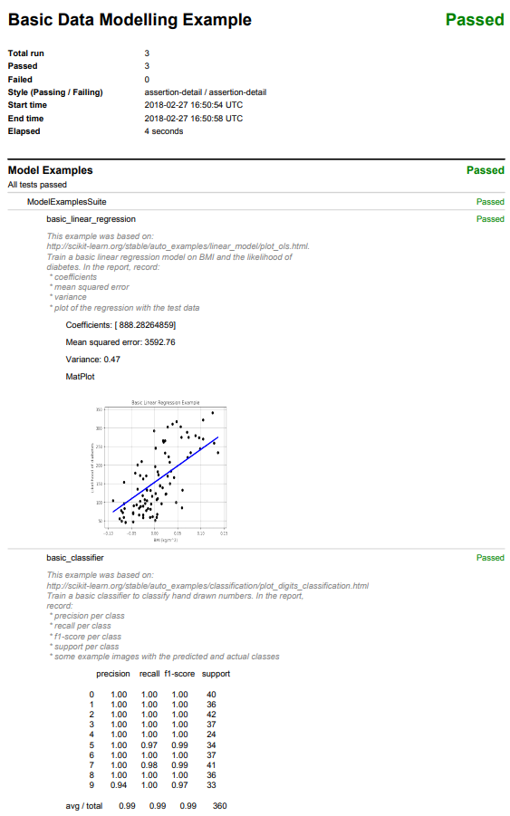
This example was based on:
http://scikit-learn.org/stable/auto_examples/linear_model/plot_ols.html.
Train a basic linear regression model on BMI and the likelihood of
diabetes. In the report, record:
* coefficients
* mean squared error
* variance
* plot of the regression with the test data
"""
# Gather and separate the data into features (X) and results (y). We are
# only using the BMI feature to compare against likelihood of diabetes.
diabetes = datasets.load_diabetes()
X = diabetes.data[:, np.newaxis, 2]
y = diabetes.target
X_train, X_test, y_train, y_test = train_test_split(
X, y, test_size=0.2
)
# Train the linear regression model and make predictions.
regr = linear_model.LinearRegression()
regr.fit(X_train, y_train)
diabetes_y_pred = regr.predict(X_test)
# Log the statistics to the report.
mse = mean_squared_error(y_test, diabetes_y_pred)
r2 = r2_score(y_test, diabetes_y_pred)
result.log("Coefficients: {}".format(regr.coef_))
result.log("Mean squared error: {0:.2f}".format(mse))
result.log("Variance: {0:.2f}".format(r2))
# Plot the predictions and display this plot on the report.
create_scatter_plot(
"Basic Linear Regression Example",
X_test,
y_test,
"BMI (kg/m^2)",
"Likelihood of diabetes",
"black",
)
plot.plot(X_test, diabetes_y_pred, color="blue", linewidth=3)
result.matplot(plot)
@testcase
def basic_classifier(self, env, result):
"""
This example was based on:
http://scikit-learn.org/stable/auto_examples/classification/plot_digits_classification.html#sphx-glr-auto-examples-classification-plot-digits-classification-py.
Train a basic classifier to classify hand drawn numbers. In the report,
record:
* precision per class
* recall per class
* f1-score per class
* support per class
* some example images with the predicted and actual classes
"""
# Gather and split the data into features (X) and results (y). We
# reshape each of the digit images from an 8x8 array into a 64x1 array.
digits = datasets.load_digits()
n_samples = len(digits.images)
data = digits.images.reshape((n_samples, -1))
X_train, X_test, y_train, y_test = train_test_split(
data, digits.target, test_size=0.2
)
# Train the classifier and make predictions.
classifier = svm.SVC(gamma=0.001)
classifier.fit(X_train, y_train)
predicted = classifier.predict(X_test)
# Log the precision, recall, f1 and supports statistics (within the
# classification report) to the report. Show four range images from the
# test set with their predictions and actual values.
result.log(classification_report(y_test, predicted))
for i, sample in enumerate(random.sample(range(0, len(y_test)), 3)):
t = "Prediction: {}\nActual: {}".format(
predicted[sample], y_test[sample]
)
create_image_plot(t, X_test[sample].reshape((8, 8)), 1, 3, i + 1)
result.matplot(plot, 4, 3)
@testcase
def basic_k_means_cluster(self, env, result):
"""
Train a basic k means cluster on some randomly generated blobs of data.
In the report, record:
* the number of clusters
* the plot of the clusters
"""
# Create random data blobs and train a K-Means cluster to group this
# data into 3 clusters.
n_clusters = 3
random_state = 100
X, y = datasets.make_blobs(n_samples=1500, random_state=random_state)
clusterer = KMeans(n_clusters=n_clusters, random_state=random_state)
y_pred = clusterer.fit_predict(X)
# Log the number of clusters and plot the clustered data.
result.log("Number of clusters: {}".format(n_clusters))
create_scatter_plot(
"Basic K-Means Cluster Example",
X[:, 0],
X[:, 1],
"Feature 1",
"Feature 2",
c=y_pred,
)
result.matplot(plot)
# Hard-coding `pdf_path` and 'pdf_style' so that the downloadable example gives
# meaningful and presentable output. NOTE: this programmatic arguments passing
# approach will cause Testplan to ignore any command line arguments related to
# that functionality.
@test_plan(
name="Basic Data Modelling Example",
pdf_path=os.path.join(os.path.dirname(__file__), "report.pdf"),
pdf_style=Style(passing="assertion-detail", failing="assertion-detail"),
)
def main(plan):
"""
Testplan decorated main function to add and execute MultiTests.
:return: Testplan result object.
:rtype: :py:class:`~testplan.base.TestplanResult`
"""
model_examples = MultiTest(
name="Model Examples", suites=[ModelExamplesSuite()]
)
plan.add(model_examples)
if __name__ == "__main__":
sys.exit(not main())
Overfitting
- Required files:
test_plan.py
#!/usr/bin/env python
# This plan contains tests that demonstrate failures as well.
"""
This example shows how to display various data modelling techniques and their
associated statistics in Testplan. The models used are:
* linear regression
* classification
* clustering
"""
import os
import sys
from testplan import test_plan
from testplan.testing.multitest import MultiTest
from testplan.testing.multitest.suite import testsuite, testcase
from testplan.report.testing.styles import Style
from testplan.common.utils.timing import Timer
from sklearn.pipeline import Pipeline
from sklearn.preprocessing import PolynomialFeatures
from sklearn.linear_model import LinearRegression
from sklearn.model_selection import cross_val_score
import matplotlib
matplotlib.use("agg")
import matplotlib.pyplot as plot
import numpy as np
# Create a Matplotlib scatter plot.
def create_scatter_plot(title, x, y, label, c=None):
plot.scatter(x, y, c=c, label=label)
plot.grid()
plot.xlabel("x")
plot.ylabel("y")
plot.xlim((0, 1))
plot.ylim((-2, 2))
plot.title(title)
# Use the original docstring, formatting
# it using kwargs via string interpolation.
# e.g. `foo: {foo}, bar: {bar}`.format(foo=2, bar=5)` -> 'foo: 2, bar: 5'
def interpolate_docstring(docstring, kwargs):
return docstring.format(**kwargs)
@testsuite
class ModelExamplesSuite:
def setup(self, env, result):
"""
Load the raw data from the CSV file.
Log this data as a table in the report.
"""
# Load the raw cosine data from the CSV file.
self.x, self.y = np.loadtxt(
os.path.join(os.path.dirname(__file__), "cos_data.csv"),
delimiter=",",
unpack=True,
skiprows=1,
)
self.x_test = np.linspace(0, 1, 100)
# Log it to display in the report, this will show the first 5 and last 5
# rows if there are more than 10 rows.
data = [["X", "y"]] + [
[self.x[i], self.y[i]] for i in range(len(self.x))
]
result.table.log(data, description="Raw cosine data")
@testcase(
parameters={"degrees": [2, 3, 4, 5, 10, 15]},
docstring_func=interpolate_docstring,
)
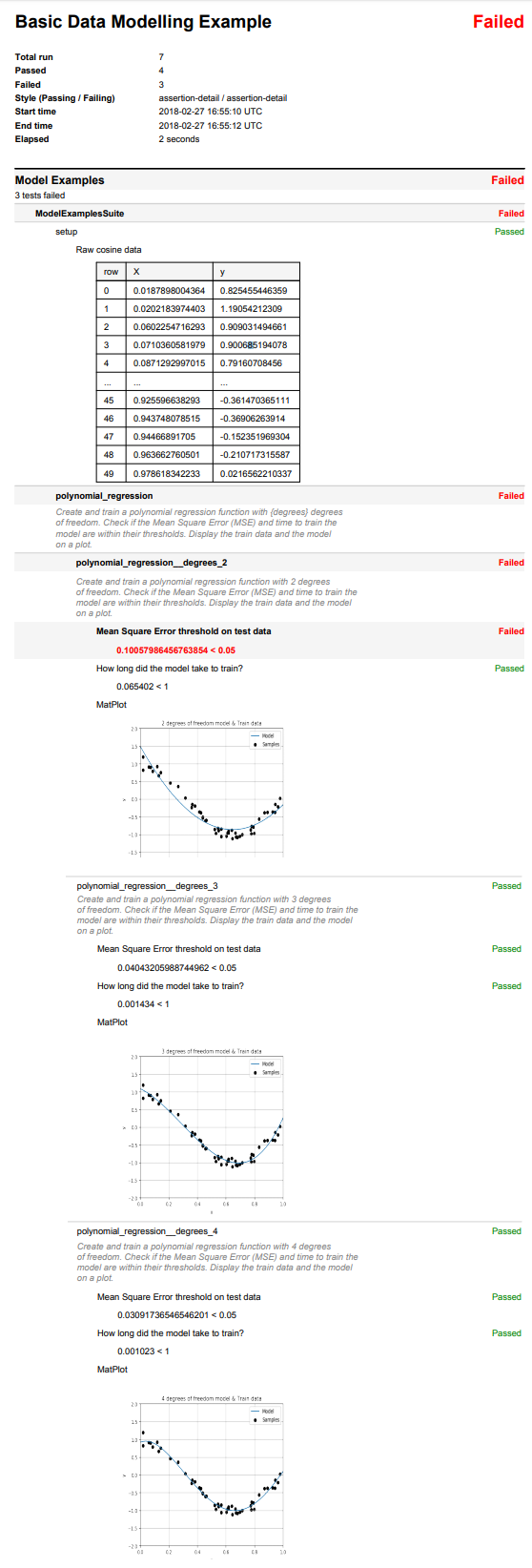
def polynomial_regression(self, env, result, degrees):
"""
Create and train a polynomial regression function with {degrees} degrees
of freedom. Check if the Mean Square Error (MSE) and time to train the
model are within their thresholds. Display the train data and the model
on a plot.
"""
# This example was based on
# http://scikit-learn.org/stable/auto_examples/model_selection/plot_underfitting_overfitting.html
# Create the pipeline to train a polynomial regression with varying
# degrees of freedom.
polynomial_features = PolynomialFeatures(
degree=degrees, include_bias=False
)
pipeline = Pipeline(
[
("polynomial_features", polynomial_features),
("linear_regression", LinearRegression()),
]
)
# Train the model and record how long this takes.
timer = Timer()
with timer.record("train_model"):
pipeline.fit(self.x[:, np.newaxis], self.y)
scores = cross_val_score(
pipeline,
self.x[:, np.newaxis],
self.y,
scoring="neg_mean_squared_error",
cv=10,
)
# Check the Mean Square Error (MSE) and time to train the model are
# within their thresholds.
result.less(
-scores.mean(),
0.05,
description="Mean Square Error threshold on test data",
)
result.less(
timer.last(key="train_model").elapsed,
1,
description="How long did the model take to train?",
)
# Display the train data and the model on a plot.
create_scatter_plot(
title="{} degrees of freedom model & Train data".format(degrees),
x=self.x,
y=self.y,
label="Samples",
c="black",
)
y_test = pipeline.predict(self.x_test[:, np.newaxis])
plot.plot(self.x_test, y_test, label="Model")
plot.legend(loc="best")
result.matplot(plot)
# Hard-coding `pdf_path` and 'pdf_style' so that the downloadable example gives
# meaningful and presentable output. NOTE: this programmatic arguments passing
# approach will cause Testplan to ignore any command line arguments related to
# that functionality.
@test_plan(
name="Basic Data Modelling Example",
pdf_path=os.path.join(os.path.dirname(__file__), "report.pdf"),
pdf_style=Style(passing="assertion-detail", failing="assertion-detail"),
)
def main(plan):
"""
Testplan decorated main function to add and execute MultiTests.
:return: Testplan result object.
:rtype: :py:class:`~testplan.base.TestplanResult`
"""
model_examples = MultiTest(
name="Model Examples", suites=[ModelExamplesSuite()]
)
plan.add(model_examples)
if __name__ == "__main__":
sys.exit(not main())
cos_data.csv
X,y
1.878980043635514185e-02,8.254554463594766522e-01
2.021839744032571939e-02,1.190542123094355809e+00
6.022547162926983333e-02,9.090314946606257163e-01
7.103605819788694209e-02,9.006851940779262433e-01
8.712929970154070780e-02,7.916070845603220274e-01
1.182744258689332195e-01,9.264061152546703148e-01
1.289262976548533057e-01,6.596588035740591494e-01
1.433532874090464038e-01,7.590975834454046778e-01
2.103825610738409013e-01,4.579684965884241454e-01
2.645556121046269693e-01,3.571530123984236194e-01
3.154283509241838646e-01,3.319464989659558912e-02
3.595079005737860101e-01,-2.410954388528686043e-01
3.637107709426226076e-01,-1.454801195509775880e-01
3.834415188257777052e-01,-1.911078724170920673e-01
4.146619399905235870e-01,-3.672868255522013792e-01
4.236547993389047084e-01,-3.826473562137094331e-01
4.370319537993414549e-01,-5.328826217219828631e-01
4.375872112626925103e-01,-5.080332597798727923e-01
4.561503322165485486e-01,-6.142335792185962262e-01
4.614793622529318462e-01,-6.037908408210926892e-01
5.218483217500716753e-01,-8.573505437373947213e-01
5.288949197529044799e-01,-9.691753605077865208e-01
5.448831829968968643e-01,-8.220522052993319839e-01
5.488135039273247529e-01,-8.898835354885372695e-01
5.680445610939323098e-01,-1.056955394776426083e+00
5.684339488686485087e-01,-8.484782439645164320e-01
6.027633760716438749e-01,-1.045729653474798848e+00
6.120957227224214092e-01,-9.619217724657304069e-01
6.169339968747569181e-01,-8.997541785724504360e-01
6.176354970758770602e-01,-9.605272878238070300e-01
6.399210213275238202e-01,-8.781279178485223991e-01
6.458941130666561170e-01,-1.118695341735484572e+00
6.667667154456676792e-01,-9.597657247408495351e-01
6.706378696181594101e-01,-1.068305910056648100e+00
6.818202991034834071e-01,-1.084531117694096158e+00
6.976311959272648577e-01,-1.047257970376244129e+00
7.151893663724194772e-01,-1.005126754505744513e+00
7.742336894342166653e-01,-8.686382664494641803e-01
7.781567509498504842e-01,-9.816460728182452300e-01
7.805291762864554617e-01,-7.693873146907472815e-01
7.917250380826645895e-01,-7.847505168286996735e-01
7.991585642167235992e-01,-9.649656670238975220e-01
8.326198455479379978e-01,-5.606550175815971926e-01
8.700121482468191614e-01,-3.853694966648019138e-01
8.917730007820797722e-01,-3.703060260261964443e-01
9.255966382926610336e-01,-3.614703651112560756e-01
9.437480785146241669e-01,-3.690626391397222594e-01
9.446689170495838894e-01,-1.523519693038673517e-01
9.636627605010292807e-01,-2.107173155867676784e-01
9.786183422327640047e-01,2.165622103369364837e-02